Finding $81.6M of unmet taxi demand in NYC with H3 and PostGIS

#The short answer

New York City's Yellow Taxi fleet loses an estimated $81.6M a year in unmet demand, and most of it sits in just 13 undersupplied zones. At the same time, 159 zones are oversupplied. The problem is not a shortage of taxis but misallocation: cars are in the wrong place at the wrong time. Moving existing supply matters more than adding more of it.

I reached this by analysing a full year of 2023 NYC TLC Yellow Taxi trips (about 35M records after filtering) on an H3 hexagon grid, then turning the supply–demand gap into a dollar figure an operations team could act on.

#Why a demand heatmap is not enough

Most taxi and ride-hailing heatmaps stop at where rides happen. That is not actionable: everyone already knows Midtown and the airports are busy. The useful operational question is the gap: where does demand keep outrunning the supply that actually shows up, and where does supply sit idle?

So every H3 cell in the city gets a position on a supply–demand axis, and the gap gets a price.

#The pipeline

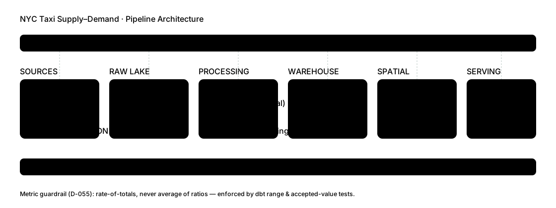Open full size

Read the diagram from left to right. Three parts carry most of the weight:

1. Ingestion and processing. The 12 monthly Parquet files come straight from the official TLC endpoint, orchestrated with Kestra. PySpark on short-lived Dataproc clusters handles the ~35M rows, the mid-2023 schema change (each file is read, cast and unioned separately) and H3 indexing.
2. Warehouse. BigQuery holds the raw data; dbt builds staging → intermediate → mart models, with data tests as regression guardrails.
3. Spatial layer and serving. PostGIS on Supabase validates boroughs with ST_Within and measures transit-hub proximity with ST_Buffer. A Streamlit dashboard shows the 2D/3D hexagon map, KPIs and a zone table. The whole stack is provisioned with Terraform on GCP.

#How supply and demand are measured

Every metric is computed per H3 resolution-8 cell (about 1,070 cells over NYC) and then rolled up to TLC zones for reporting.

• Demand = pickups in a cell. Supply = drop-offs in a cell.
• This is a pickup–drop-off asymmetry proxy, not live driver availability: a drop-off is where a driver became available, not proof they stayed. It is still a strong directional signal of where the fleet sits relative to where it is hailed.
• Cells with fewer than 500 trips a year are dropped so low-volume cells cannot game the rankings (243 → 185 reported cells).
• A ±10% band classifies each zone: a supply/demand ratio of 0.9–1.1 is balanced, below is undersupplied, above is oversupplied. Revenue loss is attributed to undersupplied zones only.

#The metric bug that almost shipped

The first version averaged per-cell ratios up to zone level. Sparse cells (for example demand = 1 and supply = 42) produced rates like −41, which poisoned the zone averages and surfaced nonsense.

The fix is simple to state and easy to forget: sum the totals first, then divide once.

-- Wrong: average of per-cell ratios (sparse cells dominate)
select zone, avg((demand - supply) / demand) as unmet_rate
from cell_metrics
group by zone;

-- Right: ratio of totals
select zone, (sum(demand) - sum(supply)) / sum(demand) as unmet_rate
from cell_metrics
group by zone;

#What the numbers say

Finding	Value
Estimated unmet demand (upper bound)	$81.6M / year
Undersupplied vs oversupplied zones	13 vs 159
JFK Airport	$26.3M (32% of the total), 79% unmet demand
LaGuardia Airport	~$15.0M
Garment District (within 800 m of Penn Station)	~$11.4M
Queens / Manhattan	~$44.0M (airport-driven) / ~$37.6M (commuter-driven)
Brooklyn and the Bronx	no undersupplied zones

The airports dominate, but the Garment District result is the interesting one: an ST_Buffer around Penn Station shows a commuter-exit gap that a borough-level view would hide.

#Is it the roads?

A natural hypothesis is that undersupplied zones are simply harder for taxis to reach. To test it, I joined 72,005 drivable OpenStreetMap segments (Geofabrik NY extract) to the zones in PostGIS.

The data says no. Undersupplied zones average 113.8 road segments versus 95.1 for oversupplied zones. Taxis avoid some of the most accessible, highest-demand zones. LaGuardia (9 segments, ~$15M lost) and JFK (192 segments, ~$26M lost) are both badly undersupplied whatever their road access. This is a dispatch and positioning problem, not an infrastructure one.

#Honest limitations

A case study that hides its caveats is less trustworthy, not more:

1. $81.6M is an estimated upper bound, not observed lost revenue. It applies an aggregate fare ratio to unmet demand; real recoverable revenue would be lower because of price elasticity and substitution.
2. Supply and demand are proxies (drop-offs and pickups), not live driver state.
3. One year, one mode: 2023 Yellow Taxi only, with no green cabs, for-hire vehicles or multi-year seasonality.
4. Spatial validation: 181 of 185 cells matched a borough polygon and 180 of those carry the right label; 4 cells sit on water or boundary edges with $0 loss. Marble Hill is administratively Manhattan but spatially in the Bronx (the Harlem Ship Canal moved it in 1895). Both labels are correct in their own frame.

#What I would tell an operations team

Rebalance before you expand. The fleet is big enough; the question is positioning. The first moves are the airport queues at JFK and LaGuardia and the commuter exits around Penn Station, where a small shift in supply recovers the largest share of the gap.

#FAQ

What is H3 and why use it for taxi data? H3 is a hexagonal grid system from Uber that splits the map into cells of equal shape. Hexagons have uniform neighbours, which makes demand and supply comparable across the city. Resolution 8 (about 1,070 cells over NYC) is fine enough to separate an airport from its surroundings and coarse enough to keep counts stable.

Why are pickups and drop-offs used as demand and supply? TLC trip records don't include live driver positions. Pickups show where riders were served, and drop-offs show where a driver became free. The gap between them is a directional proxy for where the fleet sits relative to demand.

Is $81.6M real lost revenue? No. It is an estimated upper bound: unmet demand multiplied by an aggregate fare ratio. Real recoverable revenue would be lower.

Can I explore the data? Yes. The live dashboard shows the hexagon map and zone table, and the GitHub repository contains the pipeline, the dbt models and a decisions log with 58 entries (D-001 to D-058).

---

Data: NYC TLC Yellow Taxi trip records, 2023 (full year, official CloudFront Parquet). Road network: OpenStreetMap via Geofabrik. Last updated: 20 October 2026.